
Over a decade ago I created a rogue teaching course called Data Analysis for Biologists. At that time most biologists were untrained and afraid of any kind of code. Today, things have changed, and many biologists can code which makes me immensely happy. The last decade has also seen significant advances in the field of Causality and I now believe that for biologists of the next generation understanding causality at a deep level will be critical for experiment design and data gathering.
This will be a series of posts which borrows ideas from the wonderful book “The Data Analyst’s Guide to Cause and Effect”. You should absolutely go and get and book. In this series I will be translating some of the ideas into the biological context to help us all think deeper about the underlying mechanics of how we do science.
Before we jump into things, ponder a little bit about the idea that the data which you collect does NOT contain information about the process that generated the data. That information, the causal information lies outside the data and must be taken into account when doing any kind of statistics.
My last course used the toy example of analysing images as a way to code, following that tradition this time we will also setup a toy experiment based around imaging, but really you can substitute any other data collection modality. What is important is the big picture understanding of how the data came to be.
Without further ado, let’s jump into things.
1. Experiment Setup - Does Drug A Cause Cell Death?
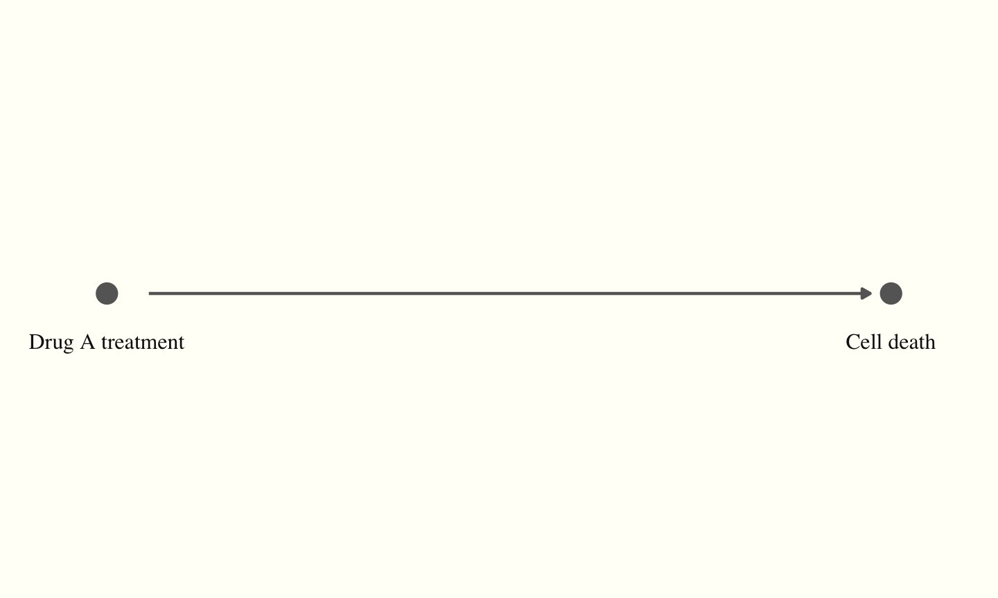
Lets take a simple experiment which is commonly performed measuring cell death after some treatment. We don’t have a whiteboard so lets draw out what that would look like if represented visually.
What you see above is the simplest version of a “DAG” or Directed Acyclic Graph. This is a simple way to represent causality. The Directed part means that one thing leads to another and Acyclic means that there are no loops things can only move in one direction. This property makes DAGs mathematically interpretable.
At first glance it might feel like this is a sufficient way to represent the treatment, what you might be disregarding is the mountain of contextual information that you carry around in your head or lab notebooks about the actual experiment.
Thus, “Does Drug A cause cell death?” is too vague to analyze. It leaves several biological decisions unspecified:
- Which cells?
- Which concentration?
- How long is the exposure?
- Compared with untreated cells, a vehicle control, or another drug?
- Is death measured at 6, 24, or 72 hours?
- Are we asking about these donors or a broader donor population?
The actual experiment would look more like this:
Primary cells from multiple donors are plated into multiwell plates. Wells are randomized to receive either Drug A or a matched vehicle control. After 24 hours, the plate is imaged using live/dead staining. Image analysis produces the number of dead and total cells in each well.
So, the first step in causal analysis is to define as well as you can the process that creates the data and to also specify the question that the experiment intends to answer. Sometimes the experiment setup can’t answer the question and it’s better to know this before you do the experiment and conitnue living in blissful, but unfortunate, ignorance.
2. Seeing the experiment at different levels
So, same as the experiment specification the question is not just “Is there an increase in cell death?” It is more along the lines of:
Among primary cell cultures from the donor population represented by this experiment, what is the average change in the proportion of cells dead after 24 hours if comparable wells receive 1 µM Drug A rather than matched vehicle?
When spelled out like this, we can start to separate out the various levels or units at which we think about the experiment. Imaging experiments often contain thousands or millions of cells. That does not mean they contain thousands or millions of independent experiments. So, cells are not included as a unit of consideration.
| Unit | In this experiment | Why it matters |
|---|---|---|
| Biological unit | Donor | Defines biological replication and the population across which effects are averaged |
| Experimental unit | Well | Receives the randomized drug or vehicle assignment |
| Blocking unit | Donor × plate | Defines the local randomization block and controls plate-specific conditions |
| Measurement unit | Segmented cell | Contributes to the measured outcome within a well |
| Technical unit | Image field or acquisition run | Can introduce focus, illumination, segmentation, and batch variation |
As we map out these units it becomes apparent that variation, noise, and importantly causes can enter the experiment from various sources. For causal approaches we need to have a good handle on these. But a list of possible sources of variation still does not tell us exactly what answer we want from the experiment. That is the job of the next step.
3. Decide exactly what you want to learn: the estimand
Before choosing a statistical test or fitting a model, we need to decide what quantity would count as an answer to our biological question. Causal inference calls this target quantity the estimand.
The word sounds more technical than it is. An estimand is a precise description of the comparison we want to make. It specifies: - who or what we want to learn about - which intervention we are considering - what it is compared with - what outcome we will measure - when we will measure it, and - how the individual comparisons will be combined
In our experiment, we expose each donor’s cells to Drug A and then also observe the vehicle control with those same cells, at the same time and under the same conditions. The causal effect for that donor would be the difference between those two outcomes. We cannot observe both versions of the same well—that unobserved alternative is the counterfactual—but randomization lets different, comparable wells stand in for those two possibilities. Our estimand is the average of those Drug A-versus-vehicle differences across the donor population represented by the experiment.
Later we will talk about two more terms but I’m noting them here in case you want some starting points to expplore with your AI:
- The estimand is the exact causal quantity we want to know.
- The estimator is the statistical procedure we will eventually use to learn it from data.
- The estimate is the number that procedure produces for this particular dataset.
At this stage we are defining the first of these. Specificying these estimands forces us to finish the scientific question before the analysis distracts us.
| Element | Definition |
|---|---|
| Population | Primary cell cultures from donors meeting the experiment’s eligibility criteria |
| Intervention | 1 µM Drug A delivered in the specified medium for 24 hours |
| Comparator | Matched vehicle delivered using the same protocol for 24 hours |
| Outcome | Proportion of successfully classified cells labeled dead at 24 hours |
| Summary measure | Average absolute difference in death proportion: Drug A minus vehicle |
| Biological averaging unit | Donor; each donor contributes equally to the final average |
| Experimental unit | Well, randomized within donor × plate blocks |
| Target interpretation | Average causal effect across the represented donor population under this protocol |
The estimands can be recomposed: among eligible donor cultures, compare 1 µM Drug A with matched vehicle after 24 hours, measure the absolute difference in the proportion of cells classified as dead, calculate that contrast within the randomized well structure, and average so that each donor contributes equally.
Each estimand is important. For example, changing from absolute difference to relative change would be a different estimand. Giving every cell equal weight instead of every donor would define a different estimand. Generalizing to donors who could never have entered this experiment — something that we’d want to do in real life — would define a different estimand. Specifying the estimands before doing the experiment allows you to argue before you actually do the experiment. Thiking is cheap, execution is expensive, so this kind of discipline also helps even if you don’t care much about causal analysis.
We’re only part way there to have a clear picuture of the experiment. The estimand tells us the comparison we want, but it does not by itself tell us whether the experiment can support a causal interpretation. For that we must state what we believe caused the treatment, the biological outcome, and the value ultimately written into the dataset.
4. Draw the causal assumptions
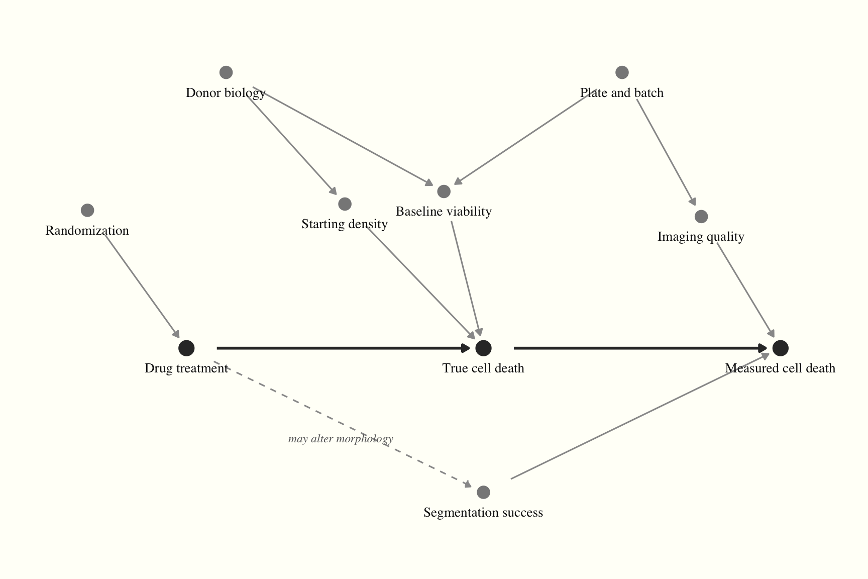
A directed acyclic graph, or DAG, is a compact way to put those beliefs on the page. It is not discovered by searching the data for strong correlations. Its arrows come from the protocol, the order in which events occur, biological knowledge, and what we know about the imaging and measurement pipeline. Which is to repeat that causal forces can’t be surmised from the data.
Drug treatment may change true cell death, and true cell death must then become measured cell death through our assay and image-analysis system. The other nodes sit above and below it to show where biological, experimental, and measurement variation can enter.
We will stop here for this post. I hope it gave you a sense that not only are there more factors that you need to consciously record but that their effects might be a source of variation which you hadn’t expected. This was a simple setup so it’s easy to see, but real experiments are more complicated and tools like DAGs help.